4 - Learning

Supervised Learning

Learning from a discrete function f (actual data) to create a function h that approximate the behavior of f.

Nearest-Neighbor Classification

Just choose the same value as the nearest neighbor.

Sometimes we can use k-nearest neighbors and choose the most common value.

Perceptron Learning

Assume f is a binary function like this:

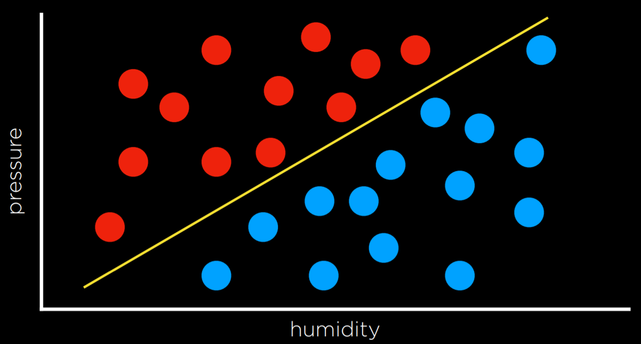
Then we can use a linear boundary to do the classification.
Assume
\mathbf{x}=(1,x_{1},x_{2}), \mathbf{w}=(w_{0},w_{1},w_{2})
Then function h can be written as
h_{\mathbf{w}}(x)=\begin{cases} 1 & \text{if } \mathbf{w}\cdot \mathbf{x}\geq 0\\ 0 & \text{Otherwise} \end{cases}
One way to find the best weight vector \mathbf{w} is to use perception learning:
w_{i} \gets w_{i}+\alpha(y-h_{\mathbf{w}}(x)) \times x_{i}
We start from a random vector \mathbf{w} and keep learning from each data point.
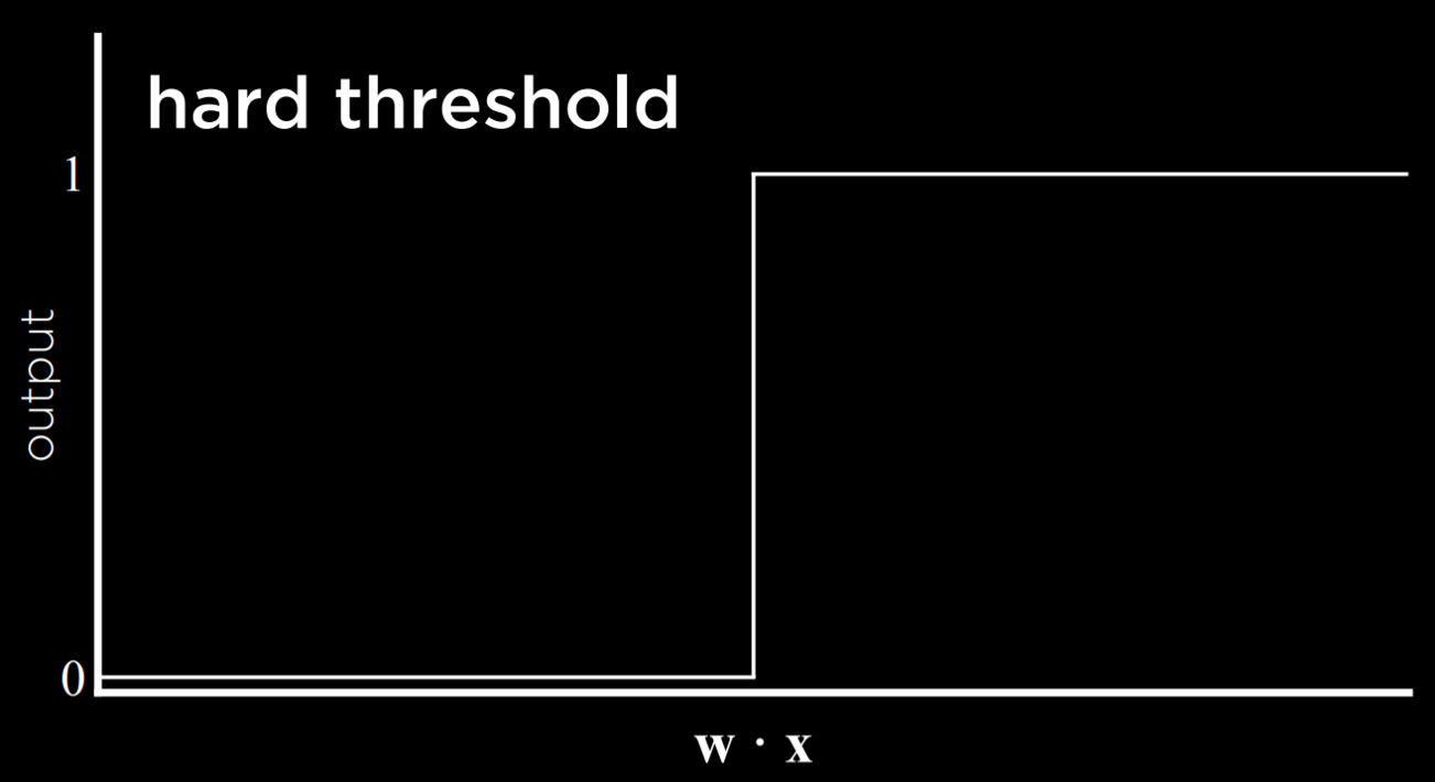
Here h is like:

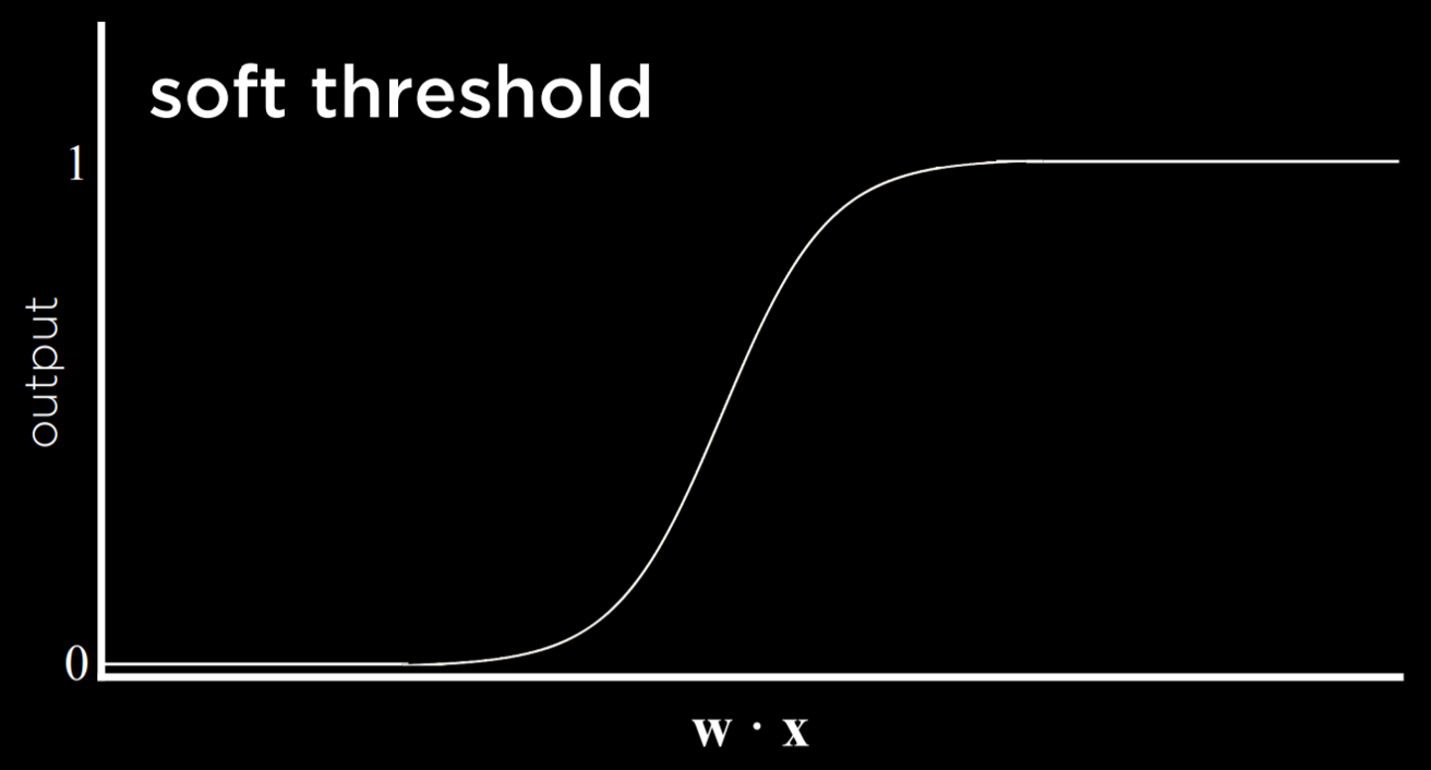
We can also make it a soft threshold:

Support Vector Machines

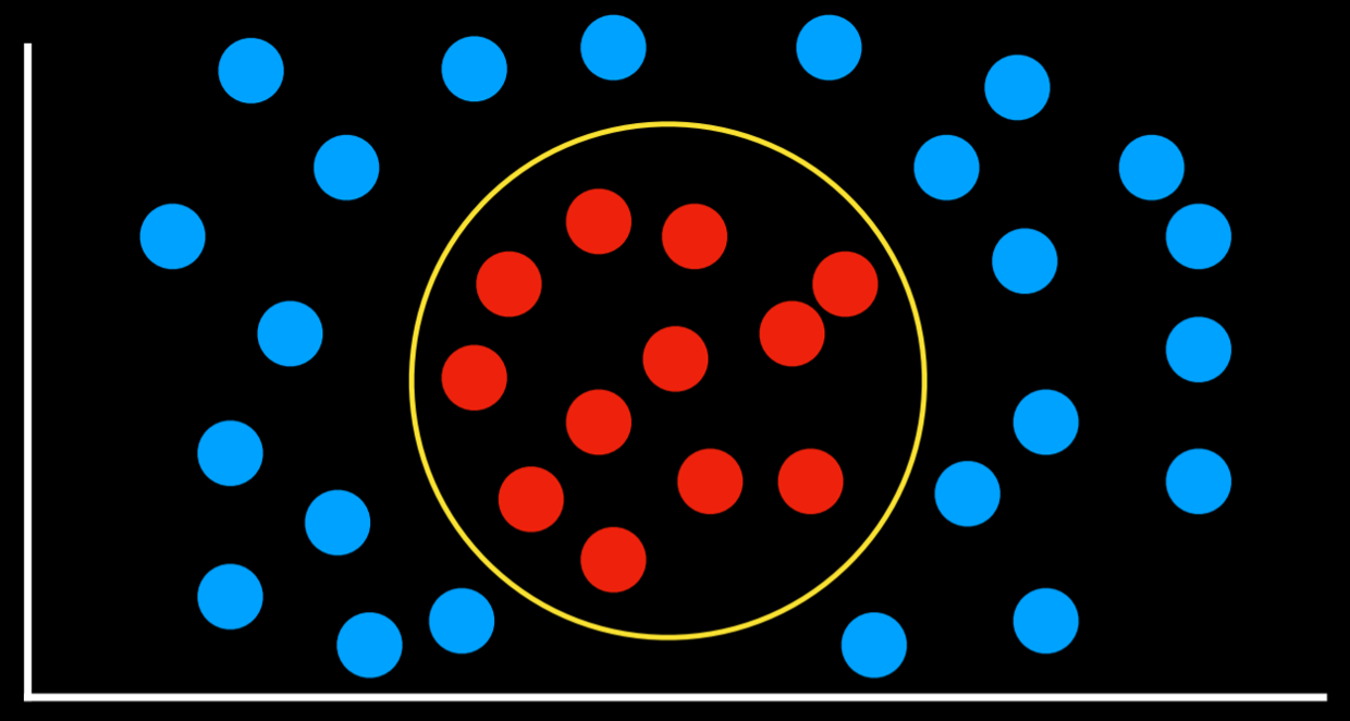
We want to find the Maximum Margin Separator(as far as possible from the two groups it separates).

Regression

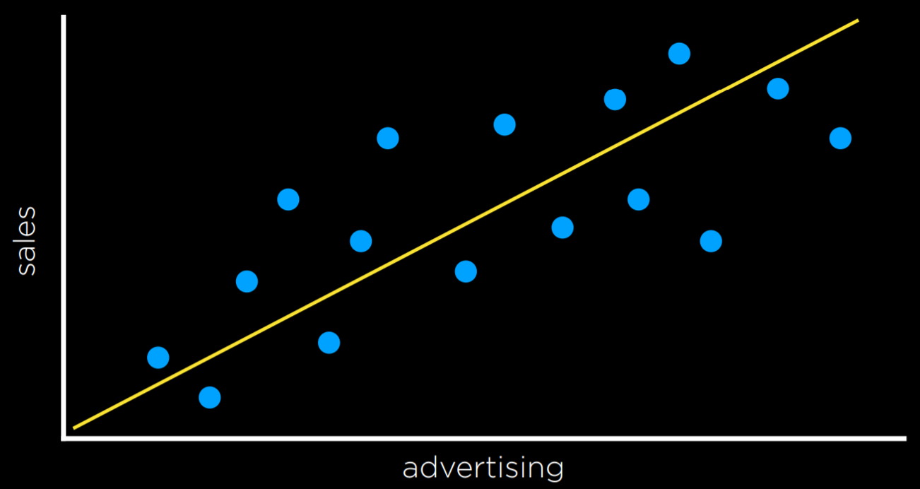
A supervised learning task of a function that maps an input point to a continuous value.
E.g. Linear regression

Loss Function

Quantifying the utility lost by the prediction.

For classification problems, it is a 0-1 Loss Function:
L(\text{actual}, \text{predicted}) = \begin{cases} 0 & \text{if actual = predicted} \\ 1 & \text{otehrwise} \end{cases}
For regression problems, it may be:
L_{1}(\text{actual}, \text{predicted}) = \lvert \text{actual} - \text{predicted} \rvert
L_{2}(\text{actual}, \text{predicted}) = (\text{actual} - \text{predicted})^{2}

Overfitting

A model fits the training data too well to generalize to other data set.

Regularization

To avoid overfitting:

1. Minimizing Cost (h)=Loss (h)+ \lambda Complexity (h)
2. Holdout cross-validation: split data into a training set and a test set
3. K-fold cross-validation: split data into k sets and experimenting k times, each time leaving out one dataset and using it as a test set

Reinforcement Learning

Given a set of rewards or punishments, learn what actions to take in the future.

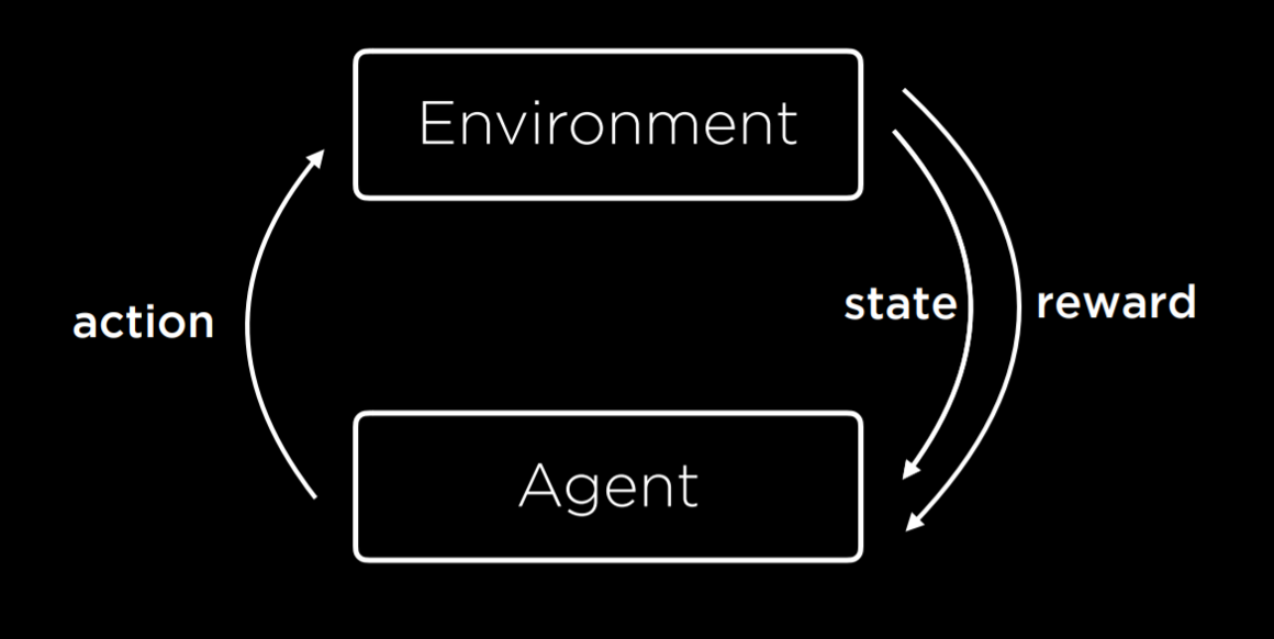
Markov Decision Processes：

• Set of states S
• Set of actions Actions (S)
• Transition model P (s’ | s, a)
• Reward function R (s, a, s’)

Q-Learning：
Q(s,a) outputs an estimate of the value of taking action a in state s.
Start with Q(s,a)=0 for all s,a.
Every time we take an action a in state s and observe a reward r, we update:
Q(s,a)\gets Q(s,a)+\alpha ((r+\gamma \max_{a'}Q(s',a'))-Q(s,a))
Here \alpha is the learning rate.

Greedy Decision-Making: Choose the maximum Q(s,a).
To let the model do some exploring, we use \varepsilon -greedy : With probability 1-\varepsilon, choose estimated best move, and with probability \varepsilon, choose a random move.

Function Approximation: to approximate Q(s,a).

Unsupervised Learning

Given input data without any additional feedback, learn patterns.

Clustering: organizing a set of objects into groups in such a way that similar objects tend to be in the same group.

K-means clustering:

Set k cluster centers.
Assign each point with the value of the closest center.
Move the centers to the middle of the corresponding points.
Keep iterating until it reaches an equilibrium.

Package: scikit learn